
I am an assistant professor of applied mathematics at the University of Warsaw, and my area of expertise lies at the intersection of two fields in the calculus of variations: optimal transport and optimal structural design. You can find out more about me here.
The goal of this webpage is to provide a concise overview of ideas I have developed together with my collaborators. I invite you to read my papers for details and to reach out with questions!
- Kantorovich–Rubinstein duality of the second order
- Optimal design of beam systems via Optimal Transport
- Zolotarev projection in convex order
1. Kantorovich-Rubinstein duality of the second order
The celebrated K-R theorem states an equality between the 1-Wasserstein distance and a supremum over the set of 1-Lipschitz potentials. V.M. Zolotarev has brought the latter formulation to higher orders. For example, given two centred probabilities \( \mu,\nu \in \mathcal{P}(\mathbb{R}^d)\) of finite second moments, the 2-Zolotarev distance reads,
\[Z_2(\mu,\nu) := \sup \left\{ \int u\, d(\mu - \nu) \ : \ u\in C^{1,1}(\mathbb{R}^d), \ \ \mathrm{lip}(\nabla u) \leq 1 \ \right\}\]K-R duality tells us that \( Z_1 = W_1 \) can be expressed via the Monge-Kantorovich optimal transport (OT) for the distance cost. In a joint paper with Guy Bouchitté we have found an OT formulation that underpins the second-order case. However, apart from the classical transport plan we also look for a vector-valued coupling,
\[Z_2(\mu,\nu) = \! \! \! \! \min_{\substack{\gamma \in\mathcal{P}(\mathbb{R}^d \times \mathbb{R}^d) \\\ q \in \mathcal{M}( \mathbb{R}^d \times \mathbb{R}^d;\mathbb{R}^d) }} \! \! \left\{ \iint \frac{1}{2}\Big(\left|\tfrac{dq}{d\gamma}(x,y)-x\right|^2 + \left|\tfrac{dq}{d\gamma}(x,y)-y\right|^2 \Big) d\gamma(x,y) \ : \ \begin{array}{l} \pi_1^\# \gamma = \mu, \\ \pi_2^\# \gamma=\nu, \end{array} \ \ \begin{array}{l} \pi_1^\# q = x \mu \\ \pi_2^\# q = y \nu \end{array} \ \right\}\]The first consequence of our new K-R-type equality is a quantitative equivalence to 2-Wasserstein distance, which we have published in our follow-up paper,
\[\frac{1}{4}\, W_2^2(\mu,\nu) \ \leq \ Z_2(\mu,\nu) \ \leq \ \frac{1}{2} \, (s_\mu + s_\nu)\, W_2(\mu,\nu)\]where \(s_\mu, s_\nu\) are the relevant standard deviations. The constants above are sharp.
Our second-order Kantorovich-Rubinstein duality is at the core of some of the topics that I expose below.
2. Optimal design of beam systems via Optimal Transport
For two probability measures \( \mu,\nu \in \mathcal{P}(\mathbb{R}^d)\) consider the minimization problem with respect to a tensor-valued measure,
\[\inf \left\{ \int \Arrowvert\sigma\Arrowvert_{\mathrm{Sch},1} : \sigma \in \mathcal{M}^b\bigl( \mathbb{R}^d;\mathbb{R}^{d \times d}_{\mathrm{sym}} \bigr), \ \ \mathrm{div}^2 \sigma = \mu-\nu \ \text{ in } \mathcal{D}'(\mathbb{R}^d) \right\}\]Above \(\Arrowvert\,\cdot\,\Arrowvert_{\mathrm{Sch},1} \) is the Schatten 1-norm, whereas \(\mathrm{div}^2 \sigma = \sum_{i,j} \partial_{ij} \sigma_{ij}\) is understood in the distributional sense. The infimum is finite and is achieved whenever \(\mu\) and \(\nu\) share the barycentre and have finite second moments.
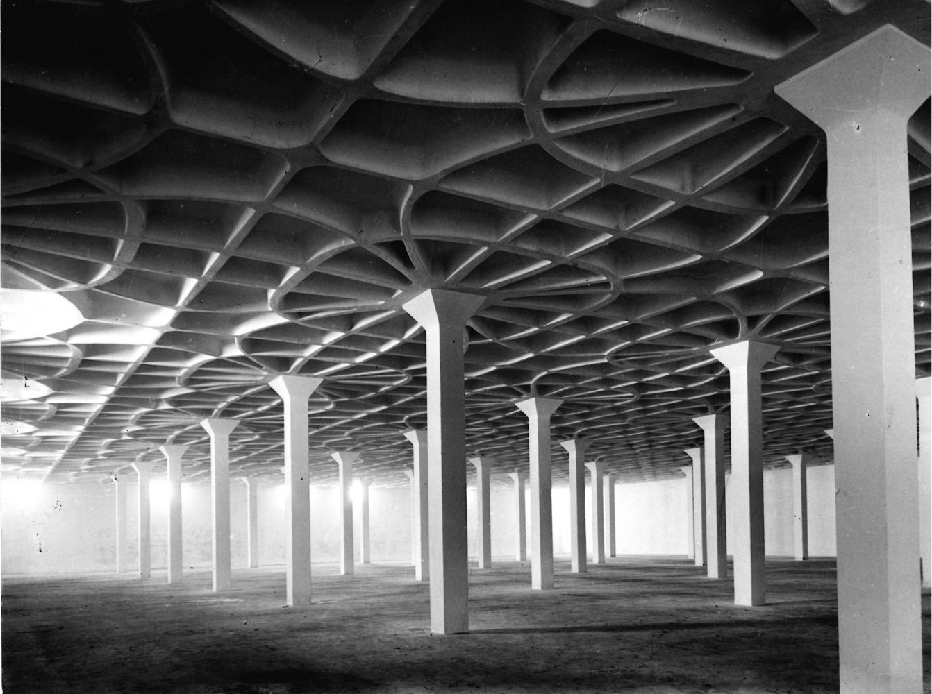
In a plane (\(d=2\)) the problem has a mechanical interpretation. Solution(s) \( \sigma \) is the bending moment tensor in the optimal (stiffest) ceiling subject to gravity forces \(\mu \) and equilbrated by the upward reaction forces \( \nu \) in the columns or walls. This design formulation builds upon the famous Michell problem and can be viewed as its plate variant.
Consider \(\sigma\) that concentrates on a 1D set. We say that such \(\sigma\) is a finite beam system or a grillage. More generally, we call the bending moment measure \(\sigma\) a beam system whenever it is a superposition of a (possibly uncountable) family of 1D tensor measures – beams.
In a paper with Guy Bouchitté we proved existence of optimal tensors \(\sigma \) which are beam systems, with the beams being polygonal chains. More precisely, for the building block we propose
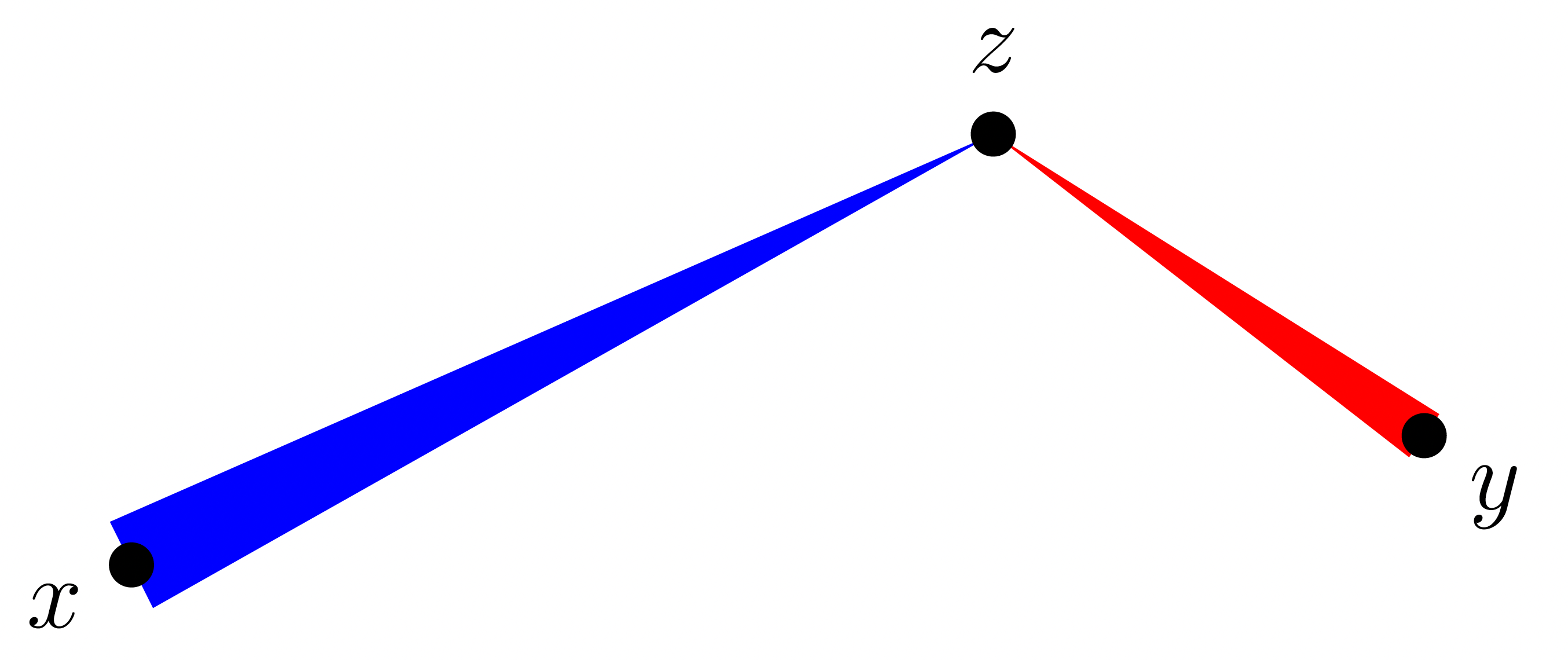
\[\sigma^{x,y,z}(\xi) := |\xi-z|\,\Big(\tfrac{x-z}{|x-z|} \! \otimes \! \tfrac{x-z}{|x-z|} \mathcal{H}^1(\xi) {\, \mathbin{\Rule{0.13ex}{1.6ex}{0ex}\Rule{1.3ex}{0.13ex}{0ex}} \, } [x,z] - \tfrac{y-z}{|y-z|} \! \otimes \! \tfrac{y-z}{|y-z|} \mathcal{H}^1(\xi) {\, \mathbin{\Rule{0.13ex}{1.6ex}{0ex}\Rule{1.3ex}{0.13ex}{0ex}} \, } [y,z] \Big)\]where \(x,y,z \) is any triple of \( \mathbb{R}^d\). This rank-1 measure concentrates on \([x,z] \cup [z,y] \), with linearly varying density that has a positive (blue) and negative (red) part:
We have shown that at least one of the optimal bending moment tensors is of the form,
\[\sigma(\xi) = \iiint \sigma^{x,y,\zeta(x,y)}(\xi) \, d\gamma(x,y)\]where \(\gamma \) is a transport plan between \(\mu\) and \(\nu\), and \(\zeta :(\mathbb{R}^d)^2 \to \mathbb{R}^d \) is a measurable coupling map. A straightforward consequence is existence of a finite optimal beam system when \(\mu,\nu \) are discrete and finitely supported. This result is in crisp contrast to the Michell problem.
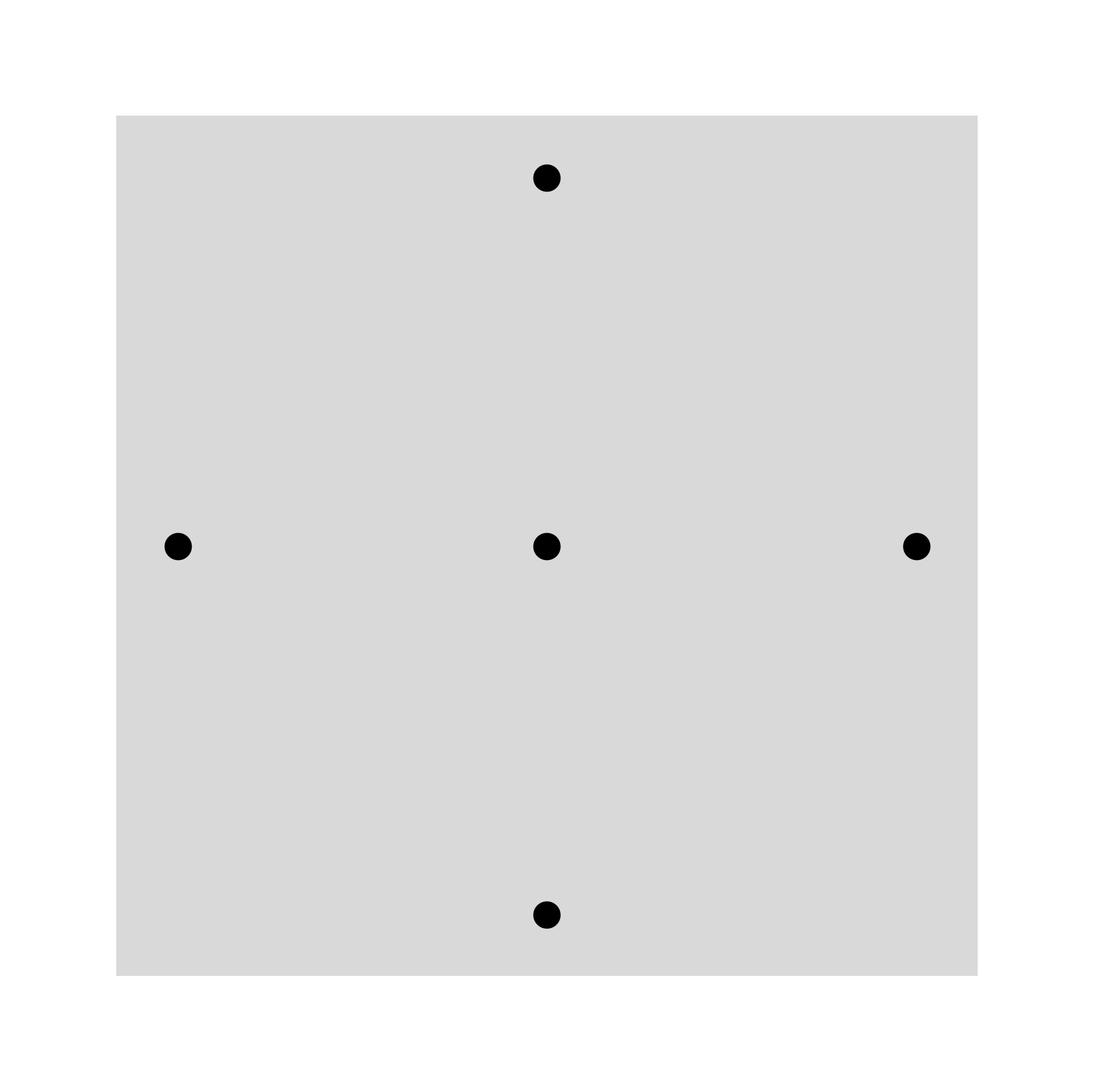
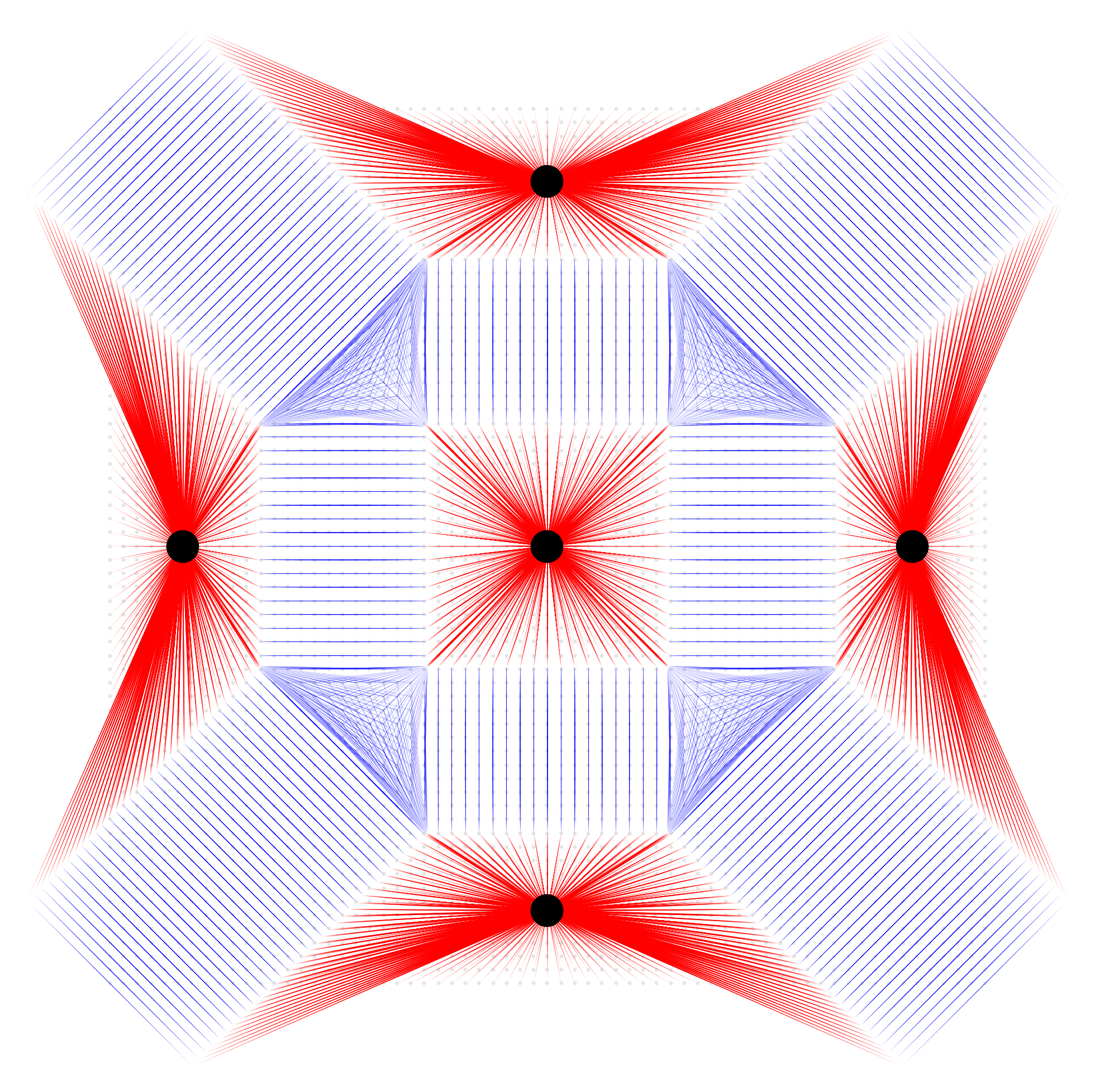
The beating heart of the new geometric insight into optimal design of beam systems is our second-order Kantorovich-Rubinstein duality. Firstly, once the condition \(\mathrm{lip}(\nabla u) \leq 1 \) is rewritten as the pointwise bound on the spectral norm of the Hessian \(\nabla^2 u \), the classical convex duality yields an equality between the minimum in \(\sigma\) and \(Z_2(\mu,\nu)\). Then, with the new transport formulation for the latter at hand, it is easy to show that its solution \((\gamma,q) \) furnishes the optimal beam system above if for \(\zeta\) one takes the Radon-Nikodym derivative \(\frac{dq}{d\gamma}\). Moreover, one can show that \(\gamma\)-a.e. there must hold,
\[\zeta(x,y) = \frac{x+y}{2} + \frac{\nabla u(x) - \nabla u(y)}{2}\]where \(u\) is any maximizing potential for \(Z_2(\mu,\nu)\).
3. Zolotarev projection in convex order
More content to come!